During my “Computational Modelling for Biomedical Imaging” course, I had the opportunity to pursue a mini-project on modeling the diffusion patterns in the brain from diffusion MRI studies. This post will give a brief overview of diffusion MRI, the models I implemented, the results, and my biggest takeaways.
Introduction to diffusion MRI
Magnetic Resonance Imaging (MRI) is a type of medical imaging modality where images of the organs are produced based on the magnetic properties of the water molecules in our body. Typically, MRI studies involve acquiring images of the organ from different views in 3D. Like images with pixels that measure the color intensity, MRI images are 3D volumes with volumetric pixels or voxels. These voxels contain information not only on the position but also the thickness of the image slice.

Diffusion MRI is a type of MRI where the intensities of the voxels are sensitive to the dispersion of water molecules. This is highly beneficial in neuroimaging research because different architectures of the nerve bundles in our brain can have different water dispersion patterns. See the image below, for example. The ventricles contain fluid that can freely diffuse in all directions, also called isotropy. But in the white matter, nerves are arranged like pipes, so water can diffuse freely along the nerves but not in the perpendicular direction, also called anisotropy. In the grey matter, the cell bodies of the nerve are clustered together so the water has isotropic diffusion as well.

By modeling these diffusion patterns from the images, we can gain valuable insights into the tissue structure and determine if there is pathology in certain brain regions.
The Data
In this project, I used the High Angular Resolution Imaging (HARDI) dataset acquired as part of the Human Connectome Project (http://www.humanconnectome.org/). It had 90 diffusion-weighted MRIs with b-value = 1000 s/mm2 and 18 MRIs with b-value=0.
Models
I investigated 4 types of models, which are discussed below:
- Diffusion tensor model – This is a straightforward model. To understand it, let’s first consider an even simpler model. We want to find the amount of diffusivity
of water in a voxel. A basic mathematical model for doing this is


where 

2. Ball-and-Stick model – This comes under a class of models called compartment models, which is really nice because it allows us to incorporate biological information about the brain. According to the Ball-and-Stick model, water diffusion in the brain can slightly vary depending on whether the water is traveling inside the nerves or outside the nerves, hence a “two-compartment” model. Water molecules outside the nerve bundles are slightly more free to move around – this is called a “ball” component. Whereas inside the axons, the water movement is more restricted to the pipe-like structure of the axon; hence this is described by a “stick” component. See how this looks in the picture below.

Overall, the equation for this two-compartment model is


which is similar to the basic model discussed earlier, with some extra terms like the 


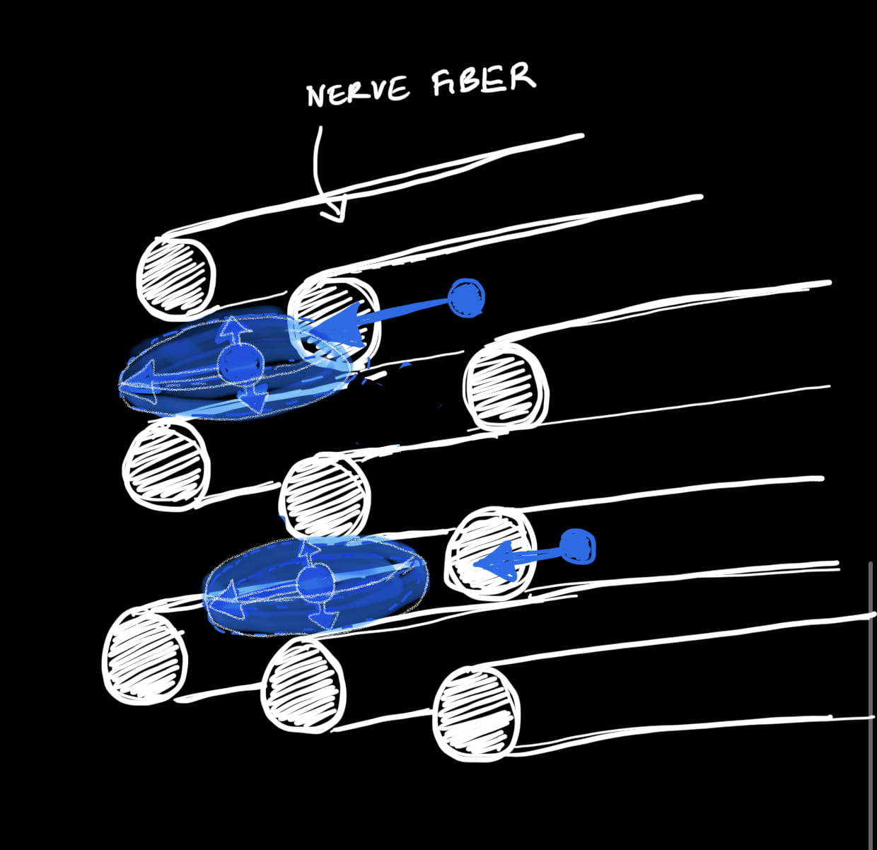
3. Zeppelin-stick model – This is another two-compartment model like the Ball-and-Stick. The difference is that instead of a Ball component, a Zeppelin component is used. The zeppelin is a structure that has the shape of an oblate spheroid. It has two principal directions (eigenvectors), where the first one has the largest eigenvalues (long axis) while the second one has the smallest eigenvalue (short axis). This model is used because we now consider that the surrounding pipe structure still restricts the water outside the nerve fibers instead of a ball-like free motion. This is visualized below.
4. Zeppelin-stick and Tortuosity – This is similar to the Zeppelin-stick with a slight modification that the principal eigenvalue is defined as a function of the second eigenvalue.
For some of these models, additional uncertainty analysis was conducted using bootstrapping and Markov-Chain Monte-Carlo. You can check this out in my code provided at the end of the article.
Results
The models above were compared using two metrics – Akaike’s information content (AIC) and Bayesian information criterion (BIC). These metrics use information about the model, specifically the number of parameters N (encodes the complexity of the model) and the log-likelihood of the data under these model parameters (encodes how well the specific model describes the data). The results are as follows:
| Model | AIC | BIC |
|---|---|---|
| Diffusion tensor | 3.8727e+03 | 1.4164e+04 |
| Ball and Stick | -1.9771e+04 | -9.4913e+03 |
| Zeppelin Stick | -2.0975e+04 | -1.0690e+04 |
| Zeppelin Stick and Tortuosity | -2.0723e+04 | -1.0444e+04 |
The Zeppelin stick model has the smallest AIC and BIC, suggesting that this model best describes water diffusion within the brain. This makes sense because it is more consistent with the nerve structure in the brain.
My Biggest Takeaways
Through this mini-project, I learned a lot about the value of computational modeling. It still surprises me is that these images, even though they are just made up of voxels, contain such valuable information that can help understand the brain. While these models were preliminary, I’m sure that further research into diffusion patterns in the brain will allow us to make them better. An exciting next step is using these diffusion maps to reconstruct the nerve pathways using tractography. This will let us create the full wiring map of the brain, also known as the connectome.
One important lesson I gained through the mini-project was model development – I started with a really simplistic model and then built up the complexity by incorporating more biological information. This is an essential strategy for model selection, as generally, the simplest model may describe the data best, so it’s always good to start basic. However, what I found challenging about the experience was that I had to program in MATLAB, which is normally the programming language of choice with such experiments and something I did not have much exposure to. With support from my professor, coursemates, and Google, of course, I developed my skills in this area. Also, while this may not be a pure machine learning project, I definitely learned a lot about concepts relevant to ML, such as basic optimization theory, determining the uncertainty in results using techniques like bootstrapping and Markov-chain-Monte Carlo. With this in mind, I hope that after my degree, I can spend some more time studying these methods in detail, especially optimization theory, as it is one of the stepping stones to developing greater machine learning algorithms.
The code for this project is on my GitHub: https://github.com/Aveturi13/Diffusion_MRI_modelling
