Automating Cardiac MR image planning using Deep Learning

Just last year, I had completed my undergraduate journey at UCL with a First Class Honors BSc in Applied Medical Sciences. As part of my degree, I got the opportunity to pursue a 9-month-long research project culminating in a dissertation. My project focused on using deep learning to automate the Cardiac MR image planning protocol.

An Introduction to Cardiac MRI

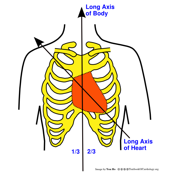
Cardiac magnetic resonance imaging (MRI) is used for visualizing the heart and evaluating various types of heart diseases like cardiomyopathy, ischemic heart disease, valvular defects and pericardial defects. Typically, what happens in the CMR protocol is the patient is passed through a huge barrel-shaped scanning machine and on the other side, technicians acquire images of the heart.

Delving a bit deeper into the imaging protocol, the first step is to acquire images in the standard anatomical views – which are the sagittal, transverse and coronal views, shown below.

Standard Anatomical Image planes. Image taken from Wikimedia Commons. https://commons.wikimedia.org/wiki/File:Human_anatomy_planes.jpg

With cardiac MRI however, there is an issue. Our heart isn’t vertically aligned, rather it lies at an angle. You can see this in the image above. Because of this tilt, the images in 3 standard views do not accurately reflect the heart’s anatomy. The solution to this is to capture the image at an angle, depending on what features have to be visualized. In imaging terminology, this is called “planning the image view”. This is a crucial step in the protocol as using the image views, radiologists will assess if there is a pathology. More importantly, from a stack of cardiac images (which is normally how CMR images are acquired), radiologists can measure how much blood is being pumped out of the heart per unit time (also called ejection fraction). This is an important metric for determining if the heart is functioning normally.

How are imaging views planned?

This a step-by-step protocol outlined in detail in cardiac MRI textbooks. Basically, the radiographer takes an initial heart image (preferably an image of the standard transverse view) and then prescribes lines on it. Using these lines as a guide, the MRI machine, “slices” the image to create the subsequent image view.

There are many possible views that can be constructed in the CMR protocol, however two imaging views are mandatory for the radiographer to capture – these are the four-chamber (4Ch) view and the two-chamber (2Ch) views. They are named so because they visualize the different chambers of the heart.

In a 4Ch view, all 4 chambers of the heart are visible and in the 2Ch view, only two are visible. To create the 4Ch view, the radiographer first prescribes a line on the transverse image, and then on the 4Ch view image, he/she prescribes another line passing through the left side of the heart (through the mitral valve and ventricular apex), slicing the image to create the 2Ch view. The workflow below shows the 4Ch view on the left and how a line is drawn (shown in yellow) to slice the image and create the 2Ch view on the right.

Creating 2-chamber view from 4-chamber view. Image taken from https://limpeter-mriblog.blogspot.com/2009/09/cardiac-localization.html

Disadvantages of the protocol

The current cardiac MRI protocol has disadvantages. Firstly, it is time-consuming, taking at least an hour per patient. Furthermore, images need to be sliced very carefully so that the cardiac features are shown correctly and the doctor can make an accurate diagnosis. This requires competent radiographers who are not available in all hospitals. Also, the process is manual which means there is a high scope for error. For these reasons, it would be beneficial if this protocol is automated. To perform this automation, deep learning would be useful. So in this project, I trained neural networks to input a 4Ch cardiac image and predict the planning line for the 2Ch image view. This hasn’t been studied much previously and because this project is just a proof-of-concept, I only focused on the 4Ch and 2Ch views, however it can be extended to more views like 3Ch and 5Ch.

My Approach to Planning Line prediction

I investigated two approaches for predicting the 2Ch planning line: these are segmentation and parameter estimation.

Segmentation

Semantic segmentation is a computer vision technique where you basically partition an image into different groups. For example, see the image below:

As you can see, there are three distinct elements in the image – the dog, the chair and the background – let’s label them as ‘class 1’, ‘class 2’ and ‘class 3’ respectively. How do we convert the original image on the left to the segmented image on the right? This is done by mapping every pixel on the original image to one of the three classes. So the pixels on the corners of the image belong to the background and will be assigned to class 3, the pixels that make up the dog will be in class 1 and the pixels for the chair will be class 2. When we view the image, we can color-code it so that pixels in classes 1, 2 and 3 will have the colors yellow, blue and red respectively. This is how we create the segmented image, also called the mask.

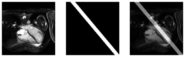
Segmentation of a cardiac image. Original image on the left. Middle image is the mask where pixels belonging to the ‘line’ class store white and pixels belonging to background store black. Right image shows the mask overlapped on the original image. Images taken from my thesis report.

This segmentation task can be performed for the 2Ch line prediction case. In the 4Ch cardiac image, pixels could be classified as belonging to one of two classes – the 2Ch line or the background. Using a supervised learning approach, I trained a convolutional neural network called the “UNet” to predict a mask for the 2Ch view and using this mask, I reconstructed the predicted 2Ch line.

Parameter estimation

This approach was simpler to implement. To perform this task, consider the property that lines can be expressed as an equation of the form

$y = mx + b$

where m and b are parameters representing the slope and the intercept respectively. A problem in using these parameters, however, is that they are unbounded values i.e. they can take any value in the range of $-\inf$ to $+\inf$ . This prevents deep learning models from learning effectively. It would be mathematically sound if the line could instead be parameterized by bounded values. To do this, I used a different equation of a line:

$r = x\cos{\theta} + y\sin{\theta}$

where $r$ and $\theta$ are the desired parameters. $r$ is the distance between the line and the origin, while $\theta$ is the angle between $r$ and the x-axis (shown below). This choice is appropriate as the angle $\theta$ can only be bounded in the range [0, 2π] while r can take values in the range [0, 160] where 160 is the size of the image. Thus, I designed a modified version of a popular neural network called the “AlexNet”, which takes the cardiac 4Ch image and predicts the values for the $r$ and $\theta$ of the 2Ch line.

r-ϴ representation of 2Ch line. Image taken from my thesis.

Training the models

For training the neural networks, I used a dataset of 600 cardiac 4Ch images and target 2Ch lines collected by Barts Cardiac Imaging centre. The targets were annotated by expert radiographers. The dataset was divided using a 75:25 split ratio where 75% of images were used for model training and the remaining 25% were used as a holdout test set to assess model predictions on new unseen data.

My Results

Overall, I found that the semantic segmentation approach was much more effective than the parameter estimation approach. You can see this in the sample test images below for each type of model. The expected 2Ch line is shown in red while the blue line is the predicted 2Ch line from the neural network.

Predictions from parameter estimation model. Images taken from my thesis report.

Predictions for segmentation model. Images taken from my thesis report.

You can see that the 2Ch line predicted by the segmentation model is pretty close to the true line. I validated this by also calculating the distance between the true and predicted 2Ch lines from each model. For the segmentation model, the average distance between the lines was 5.7mm while it was 30.2mm for the parameter estimation model.

The reason why the segmentation approach worked better was probably because the UNet has a complex autoencoder architecture which can learn the key anatomical landmarks on the 4Ch cardiac images, which is required for constructing the 2Ch line. The parameter estimation model, however, wasn’t able to learn this due to a less complex architecture, hence couldn’t perform well.

Reflecting on my experience

The results aren’t perfect and there is still room for improvement. But overall, this has been a challenging and fun project for me. Reflecting on my experience, I would say that this project actually gave me the feel of what real deep learning work involves. Prior to this project, I did pursue online courses where I could do code assignments, however these assignments mostly involved filling in code which others have already written. On the other hand, this project gave me the opportunity to tackle a real problem, experience the process of writing and debugging full programs and most importantly, clean and process raw data, which is what practitioners actually spend 90% of their time on! Alongside this, I was able to learn more about cardiac imaging and MRI acquisition from experts at Barts Cardiac Imaging Centre.

With this project, my passion for working in the medical AI field has grown. I’m excited about the opportunity to learn more about deep learning during my Machine Learning masters course, interact with experts in the field and participate in more awesome projects!

This project was executed on Google Colab, a cloud-based Jupyter Notebook service provided by Google. Do check out the Colab notebooks on my GitHub page for the source code. My final thesis report is also accessible in this repository.