
I’m sure most of us will know that proteins play a huge role in the human body. They are responsible for the metabolic reactions in our cells, carry molecules from one part of the body to another, mediate cellular repair, and form a part of our immune system. But to figure out what a protein’s function is in the first place, we need to obtain some information about it. One crucial piece of information is a protein’s subcellular location, as it can tell us what cell pathways it’s involved in and how it is connected to a disease.
Broadly, we can classify proteins into four types based on the sub-cellular location:
- Cytoplasmic proteins – From biology 101, you’d remember that the cytoplasm is the thick solution that fills a cell, and it’s where all the organelles and molecules are floating. Proteins present in the cytoplasm are generally involved in regulating metabolic reactions or acting like cargo transporters – for example, the kinesin protein shown above.
- Extracellular proteins – These proteins are secreted from the cells. For example, the pancreas secretes digestive enzymes, which break down the food we eat into basic sugars, fats, and amino acids, which get absorbed into our bloodstream.
- Nuclear proteins – The nucleus of the cell contains the genome – our DNA. So it naturally means that nuclear proteins are related to processes like DNA replication, transcription, activating/silencing genes. A famous example of this is the estrogen receptor, which binds to the estrogen hormone and forms a dimer that activates DNA transcription.
- Mitochondrial protein – The mitochondrion is the powerhouse of the cell. Therefore, mitochondrial proteins are associated with processes that generate energy. The CS protein, for example, is involved in the Krebs cycle – a pathway in aerobic cellular respiration.
But how did we find out what these proteins do and where they are located? We did it in the lab with a microscope – scientists tag these proteins with fluorescent molecules like GFP (green fluorescent protein) and, using microscopy, tracked down where these proteins are in the cell. While this has worked well, it is a time-consuming procedure. Over the past couple of years, due to the accumulation of protein data in bioinformatics databases, people have been developing computational approaches that could automate the process, particularly AI and machine learning (ML)-based approaches. As part of my bioinformatics module, I did a brief study investigating ML methods to predict a protein’s subcellular location. Specifically, we were given a dataset of protein sequences (amino acid sequences) and their actual locations. The goal was to design a model that could classify new unseen protein sequences into one of the four locations.
My approach
I thought it would be interesting to compare a classical ML algorithm to a SOTA one, so I decided to try out a support vector machine and a deep neural network. I’ll briefly outline how these two models work below:
Deep Neural Network
Neural networks have been popularly used for many tasks like object detection, facial recognition, image segmentation, disease classification, etc. These are essentially complex non-linear functions for which parameters are learned by minimizing a loss function representing the difference between the actual label and the predicted label. For a more detailed explanation, do check out my article Deep Learning Demystified.
Neural networks are highly flexible and have many hyperparameters which are tuned to improve training efficacy. In general, these models are tuned in two ways: first is the architecture of the network itself, where adding more layers can increase the number of learnable parameters and, thus, the model complexity. The second way is tuning the parameter optimization, which involves selecting the optimizer itself, its learning rate, the batch size during training, and many others. Because neural nets are flexible, they could also overfit the training data, which we deal with using regularization methods like Dropout and L2.
Support Vector Machine
The support vector machine (SVM) is a supervised learning algorithm that aims to find an optimal separating hyperplane that maximizes the margin between two data classes. To deconstruct what this means, let’s consider a toy example:
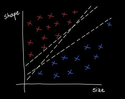
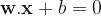
Suppose we want to predict if a tumor is benign or metastatic based on its size and shape. The plots above show some toy data on this: the axes are the shape and size of the tumor, and the red points = metastatic tumors and blue points = benign tumors. Clearly, you can see that the data is separable by a line or decision boundary such that if a new tumor falls somewhere between the red points, we classify it as metastatic, and if it falls between the blue points, then benign. But there are many possible decision boundaries I could pick to separate the data, shown as the dotted white lines. The goal is to find the optimal line or hyperplane that separates the data classes. As you may recall from high school math, a line has the equation 


Now how do we find the OSH? Well, as I said, different lines can separate the data, the best one seems to be the one that is furthest away from both classes, right? This the green line in the image above. This “far-ness” is defined by the margin. Therefore, the OSH is the one that maximizes the margin. I’ll not delve into the mathematical nitty-gritty, but in short, we find the OSH by formulating a constrained optimization objective function that is solved with Lagrange multipliers and quadratic programming methods. Do check out this fantastic Caltech lecture if you’re interested in exploring deeper.
Finally, let’s consider what do we do if the data is not linearly separable, like in the diagram below?

Here, the data shows that even though there is a distinction between metastatic and benign tumors, there are some exceptions: inter-dispersed blue and red samples. In this situation, we could use a particular type of SVM called a soft-margin SVM. The soft margin means that the SVM won’t try so hard to find that line that separates all data points perfectly; rather, it will cut some slack and allow some data points to fall on the opposite side of the boundary. In addition to this, we could incorporate kernel functions. These are functions that can expand the dimensionality of the data to create something that is linearly separable. The objective functions in these cases are also solvable using Lagrange multipliers and quadratic programming, and if you’re interested, I’d be happy to cover it in a future post! For now, I’m only applying these ideas to the protein subcellular location prediction task.
My Experiment
For my experiments, I used a dataset of around 11,000 protein sequences from the four subcellular locations listed earlier. The dataset also included sequences that aren’t in any of these locations as a “control” class. From these 11,000 proteins, 80% were used for training the models while the remaining 20% were used for testing.
Protein sequences are represented by a long string of letters, which are amino acids. There are 20 types of amino acids, which all have different biochemical properties. To process the dataset of protein sequences in a way that is interesting for biological analysis, I used the BioPython library. This library has functions to compute biochemical properties for an input sequence, like the molecular weight, isoelectric point, global amino acid composition, local amino acid composition, aromaticity, instability index, and grand-average-of-hydropathy (GRAVY). I used all these features to train both the SVM and neural network models. To arrive at the best configurations for these two models, I also performed a series of grid search + cross-validation sub-experiments, which you can read about in my final report attached below.
I trained the SVM in scikitlearn and the neural network in PyTorch.
Results
From my experiments, I found that the best SVM and neural network models had the configurations and results stated below:
| Model | Configuration | Mean cross-validation error (accuracy) ±STD | Test set Accuracy |
| SVM |
kernel = 'rbf' C = 10 gamma = 2^-7 |
0.66532 ±0.00657 | 0.6783 |
| Neural Network |
Layers = [45, 32, 5] learning_rate = 1e-4 batch_size = 128 epochs = 300 optimizer = Adam loss = cross entropy |
0.6760 ±0.02658 | 0.6532 |
I also create confusion matrices which show how many correct/incorrect classifications the models make on test set examples. The matrix diagonals contain the number of correct classifications, and the off-diagonals are the “confusions.”
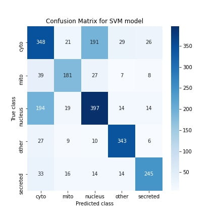
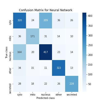
Using these confusion matrices, I also computed other scores like the precision, recall, and F1 scores, summarizing the model performance. Overall, most of the metrics were similar for both models, but the SVM showed better performance. This is quite nice because it suggests that a classical approach that needs relatively lesser hyperparameter tuning performs just as well as a SOTA approach like neural nets. Therefore one lesson I’ve gained from this is that when performing ML experiments in the future, it’s always good to start with the classical techniques.
Regardless of the models, the accuracy is still poor (~67%). A significant contributor to this is that both models confused nuclear proteins with cytoplasmic proteins, which you can see in the confusion matrix. I also measured the confidence levels of the predictions on the test set and found that both models were unsure between these two classes for nuclear and cytoplasmic sequences, which validates this. A potential reason for this mix-up is because both the nuclear and cytoplasmic proteins have similar biochemical features. I found this from studying these two classes in the dataset.
Conclusions
Overall, the performance is sub-optimal and more analysis is required. Reflecting on my experiment setup, one problem with my approach was that I used biochemical features computed from the original protein sequences to train my models. This transformation from raw data to a set feature space could result in some information loss. Therefore, a different approach could be to use the raw sequence data itself to train models. This can be achieved with NLP techniques. Especially transformer models are gaining popularity now as they can easily learn long-range dependencies, which can help analyze protein sequences at the amino acid level itself!
The report for this project can be accessed below:
[embeddoc url=”https://machinelearningandme.files.wordpress.com/2022/01/63281-comp0082_17056549.pdf” download=”all” text=”Report” viewer=”google”]
